Run OpenQASM Circuits on Your Quantum Chip

In this blog post, we present an efficient way to convert your OpenQASM3-based quantum circuits to pulse generation from your quantum control hardware through LabOne Q.

Recent advancements in qubit architectures (i.e. long qubit lifetimes, short gate times and high gate fidelities) enable modern quantum processors to run longer and more complicated quantum algorithms than what was previously possible. OpenQASM is a quantum assembly language that provides users a convenient interface to design their quantum experiments and algorithms by programming sequences of parameterized quantum operations (i.e. gates, measurements, and resets) using the quantum circuit model [1,2]. To implement experiments with a quantum processor, the quantum circuits defined through OpenQASM need to be effectively converted into language that FPGA based control electronics can understand.

LabOne Q, our software framework for quantum computing, provides the functionality for this conversion out of the box. LabOne Q assumes the role of a backend for QASM, in that the qubits and gates are defined within LabOne Q. Importing an OpenQASM program then amounts to mapping the QASM expressions to the LabOne Q objects, thus creating a pulse sequence from the QASM code that is directly executable through Zurich Instruments' Quantum Computing Control System (QCCS).

In this blog post, we walk you through the process of importing your OpenQASM quantum circuit into LabOne Q.  As an example we will work with a quantum protocol essential for quantum operations: two-qubit Randomized Benchmarking (RB). Using LabOneQ, we demonstrate how a two-qubit RB experiment is converted from OpenQASM 3 code into a pulse sequence played on an SHFQC and HDAWG. The concepts used for this example can be readily applied to other use cases, such as implementing variational quantum eigensolvers, or running custom algorithms. The full code for this example is available on our GitHub.

Starting point: the quantum circuit

Generation of OpenQASM code can be simplified through a higher level language such as Qiskit. Below we use the Qiskit experiment library to create a standard two-qubit RB experiment with varying Clifford lengths – a short example of length two is shown in Figure 1. Other languages such as pyGSTi can also be used to create an OpenQASM experiment with same functionality (an example from our GitHub can be found here).

# Use Qiskit Experiment Library to Generate RB
qiskit_experiment = randomized_benchmarking.StandardRB(
    physical_qubits=[0, 1], lengths=[2, 4, 8, 12]
).circuits()
qiskit_experiment[0].draw("mpl")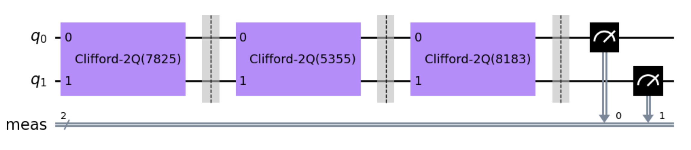

Qiskit Tools

After generating our circuit, we only need two additional tools from Qiskit. The first is Qiskit’s transpiler. Using the transpile() function, the Clifford gates shown in Figure 1 are expressed in terms of a chosen basis. Here we have chosen the Identity (id), √X (sx), X (x), R_Z (rz) and Controlled-X (cx) gates to be our basis but you can choose any set of basis gates so long as the set is universal. The transpiled circuit is shown in the top half of Figure 2.

# Choose basis gates
transpiled_circuit = transpile(
    qiskit_experiment, basis_gates=["id", "sx", "rz", "x", "cx"]
)
transpiled_circuit[0].draw("mpl")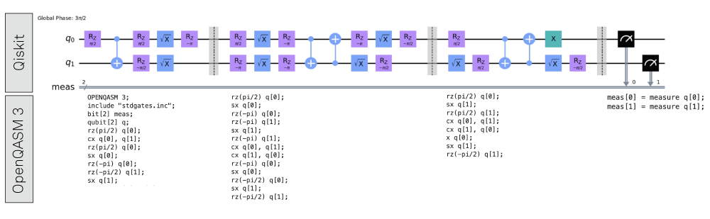

Finally, we convert our transpiled circuit into an OpenQASM 3 program. We will work with the two-qubit RB experiment seen in Figure 1 (corresponding to program_list[0] from the code below). The bottom half of Figure 2 shows the OpenQASM code that corresponds to the section of the circuit directly above it in the figure.

program_list = []
for circuit in transpiled_circuit:
    program_list.append(qasm3.dumps(circuit))
print(program_list[0])

The LabOne Q Backend

\(DR=20\log_{10}{\left(\frac{V_d}{V_s}\right)}\)

The backend for LabOne Q defines each component of a quantum circuit (qubits, basis gates and measurement sequences) in terms of the pulses associated with the respective component. Here we use the circuit depicted in Figure 2 as an example. With the help of the backend, we can map the OpenQASM code to a domain specific language (DSL) experiment or a sequence of pulses in LabOne Q

Typically, objects in the backend will take one of three forms: qubits object, individual pulses, and functions that return a LabOne Q section (we call these types of objects “section factories”). Qubit objects are the qubits you plan executing the quantum circuit on.

Individual pulses will usually correspond to single-qubit gates. For instance, a √X gate acting on qubit 0 could take the form of a DRAG pulse:

def q0_sx_gate():
    """Pulse definition for an sqrt(X) gate on qubit 0"""
    return pulse_library.drag(uid="q0_sx", length=50e-9, amplitude=0.6)

Since pulse level control is a fundamental feature of LabOne Q, you can choose any pulse from our pulse library, or define a custom pulse using a numpy array to assign to a gate. In general, it can be advantageous to specify different pulses for each qubit and operation (i.e. sx q[0] ≠ sx q[1]) so we recommend generalizing these backend definitions:

def drive_pulse(qubit: Qubit, label, length=None, amplitude=None):
    """Return a drive pulse for the given qubit. """
    
    if not length:
        length = qubit.parameters.user_defined["pulse_length"]
        
    if not amplitude:
        amplitude = qubit.parameters.user_defined["amplitude_pi"]
        
    return pulse_library.drag(
        uid = f"{qubit.uid}_{label}",
        length = length,
        amplitude = amplitude
    )

Almost all other backend objects (multi-qubit gates, single-qubit gates composed of more than one pulse, measurements, etc.) will be section factories. These objects leverage LabOne Q’s section functionalities to control the relative timings of pulses, ensure line synchronization and implement classical feedback. The measurement object shown below is an example of a section factory. 

def measurement(qubit: Qubit):
    """Return a measurement operation of the specified qubit."""

    def measurement_gate(handle: str):
        """Perform a measurement.

        Handle is the name of where to store the measurement result. E.g. "meas[0]".
        """
        gate = Section(uid=id_generator(f"meas_{qubit.uid}_{handle}"))
        gate.reserve(signal=qubit.signals["drive"])
        gate.play(signal=qubit.signals["measure"], pulse=measure_pulse)
        gate.acquire(
            signal=qubit.signals["acquire"],
            handle=handle,
            kernel=integration_kernel,
        )
        return gate

    return measurement_gate

Mapping Between LabOne Q and OpenQASM

Once the LabOne Q backend has been established, we need to map individual objects in the backend to their OpenQASM definitions. The process of mapping OpenQASM code to the LabOne Q backend is depicted in Figure 3. 

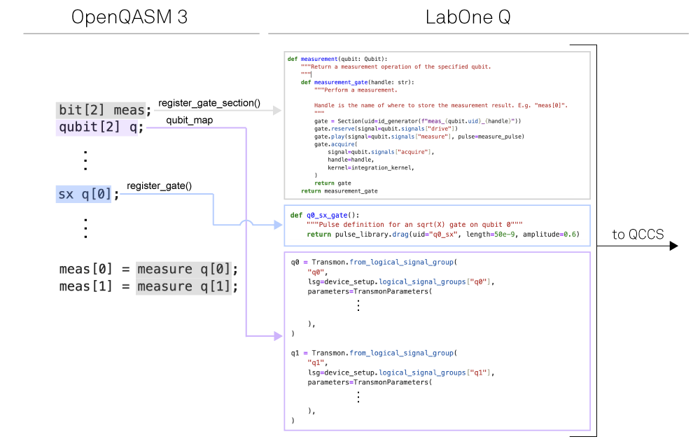
Mapping the qubits (shown in purple in Figure 3) is done using a qubit_map - a dictionary specifying which OpenQASM qubit corresponds to which LabOne Q qubit object.

qubit_map = {"q[0]": q0, "q[1]": q1}

To map gates we will use the GateStore() – LabOne Q’s class designed to hold the individual pulses and section factories we defined in our backend and the mappings of these objects to the corresponding OpenQASM circuit elements. The GateStore() is instantiated like any normal class:

gate_store = GateStore()

To map individual pulses we use the register_gate() method. We can use the q0_sx_gate() we defined previously to see how this method works. This mapping is shown in blue in Figure 3. 

gate_store.register_gate(
		"sx",
		"q[0]",
		q0_sx_gate(),
		signal=q0.signals["drive"],
	)

The first argument in the register_gate() method is the name of the OpenQASM circuit element we want to map our pulse to. The second argument is the OpenQASM qubit the pulse is played on. The third and fourth arguments are: the pulse we defined in our backend and the experimental signal line we want that pulse to be played on, respectively.

We use the register_gate_section() method to register a section factory in our gate_store (shown in gray in Figure 3). Using our measurement() object as an example:

gate_store.register_gate_section("measure", "q[0]", measurement(q0))

We see that the register_gate_section() method takes three arguments. Similar to the register_gate() method, the first two arguments are the OpenQASM circuit element and qubit we wish to map to. The third argument is the section factory we are assigning to the circuit element. Section factories already contain information about experimental signal lines and relative timings of experimental pulses so we don’t need to specify any of that information here.

Running your experiment

The final step is to generate your experiment and run it! Experiment generation is done using using the function exp_from_qasm():

exp = exp_from_qasm(program_list[0], qubits=qubit_map, gate_store=gate_store)

This function takes three arguments and returns a LabOne Q experiment object. The first input argument is the name of the OpenQASM program you want to convert into a LabOne Q experiment object. The second is the qubit map and the third is the GateStore for that particular program.

If you are interested in batch processing a list of OpenQASM programs, the function exp_from_qasm_list() can be used instead. This function is similar to exp_from_qasm() but takes a list of OpenQASM programs as the first argument. The list is processed into a single LabOne Q experiment that executes the QASM snippets sequentially. For full details on this function, see our documentation.

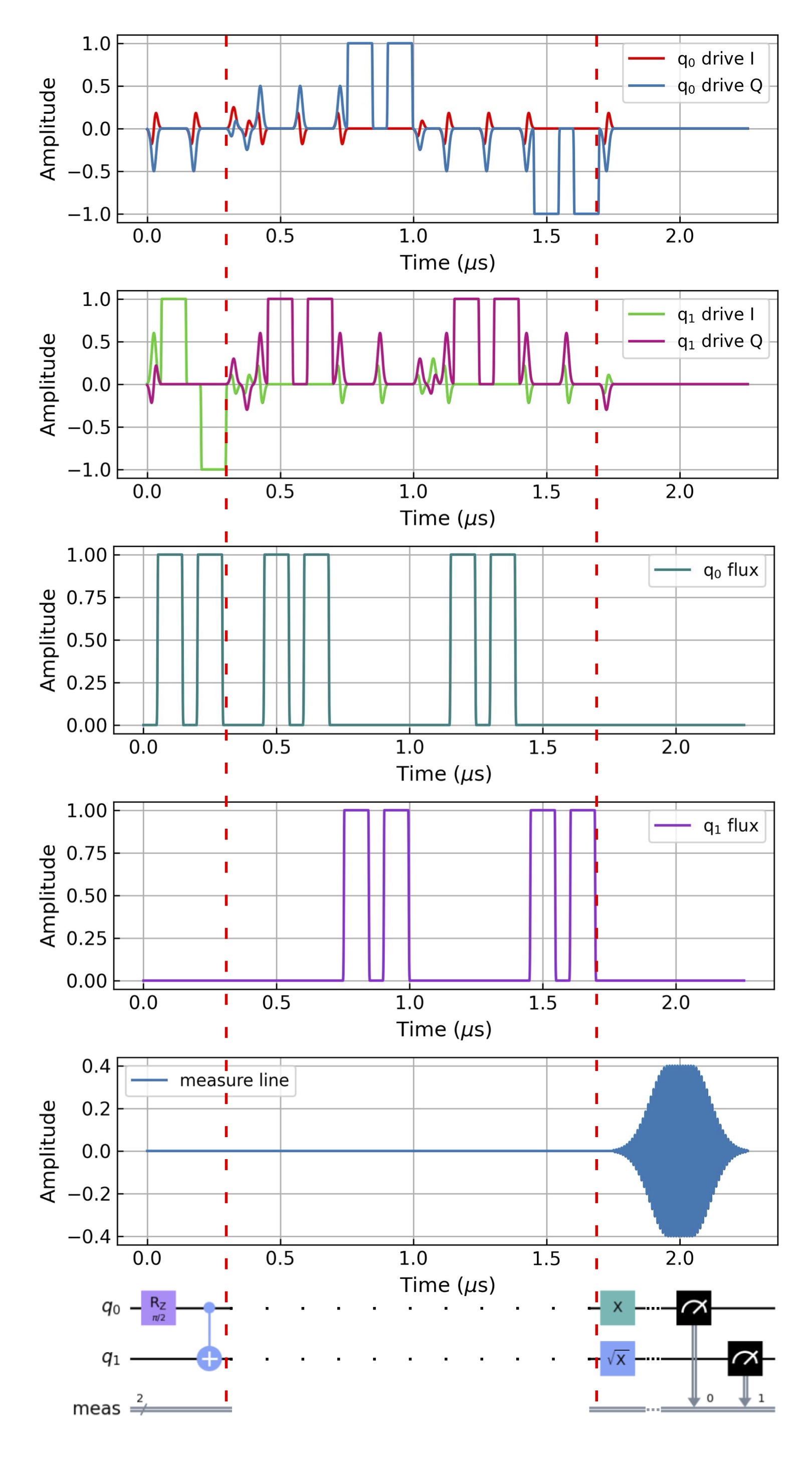
Once the experiment has been generated, it can be compiled through the LabOne Q compiler, and then executed via the QCCS hardware. Using LabOne Q's built-in simulation tool, we can preview the expected flux, drive, and measurement pulses produced by the SHFQC and HDAWG. Figure 4 shows the pulse simulation for the two-qubit RB experiment from Figure 2.

Summary

In this blog post we have used a two-qubit RB experiment written in OpenQASM code to demonstrate the quantum circuit import features of LabOne Q. LabOne Q’s qubit objects, pulse library, and section functionalities make establishing a backend for your experiment straightforward. After mapping your OpenQASM code onto the LabOne Q backend, generation, simulation and execution of your experiment on Zurich Instruments' QCCS can be completed in seconds.

Further OpenQASM support from LabOne Q, including sweep functionalities and openPulse integration, will be discussed future blog posts, so stay tuned!

Do you have a quantum circuit you want to run in your lab? We are excited to help make that happen! Write to us at Linsey.Rodenbach@zhinst.com and Taekwan.Yoon@zhinst.com.

References

1. Andrew W. Cross, Ali Javadi-Abhari, Thomas Alexander, Niel de Beaudrap, Lev S. Bishop, Steven Heidel, Colm A. Ryan, John Smolin, Jay M. Gambetta, Blake R. Johnson "OpenQASM 3: A broader and deeper quantum assembly language", ACM Transactions on Quantum Computing, 3, 3 (2022), pp 1-50
2. Introduction to OpenQASM | IBM Quantum Documentation